Tutorial

In the following we will demonstrate the epmatools package. It is currently capable of doing just few impressive things:

from epmatools import *

Basic usage

We should start with importing some data as oxides in wt%. You can use Oxides methods from_excel() or from_clipboard(), but for now we will use some example data provided:

d = Oxides.from_examples('minerals')
d

Oxides: Compo [wt%] - Original data

	SiO2	Al2O3	MgO	FeO	MnO	CaO	K2O	Na2O	TiO2	Cr2O3	ZnO	P2O5	Y2O3
0	37.218	20.349	13.784	13.140	0.000	0.013	8.998	0.404	1.010	0.022	0.020	0.005	0.007
1	37.363	20.037	14.106	12.539	0.000	0.013	8.946	0.461	1.206	0.020	0.042	0.000	0.000
2	23.748	22.152	9.611	31.549	0.066	0.028	0.023	0.035	0.047	0.000	0.017	0.037	0.000
3	46.986	39.183	0.151	1.264	0.033	0.410	3.409	4.883	0.083	0.000	0.000	0.006	0.000
4	48.389	32.414	8.227	7.713	0.060	0.027	0.000	0.924	0.005	0.009	0.000	0.005	0.000
5	48.870	32.696	8.390	7.482	0.068	0.049	0.000	0.845	0.000	0.000	0.000	0.000	0.000
6	61.839	24.661	0.000	0.484	0.015	5.738	0.032	7.917	0.000	0.010	0.019	0.025	0.000
7	37.816	21.184	4.189	35.118	1.001	1.435	0.000	0.000	0.000	0.000	0.000	0.006	0.000
8	37.584	21.311	4.651	33.895	0.999	1.454	0.000	0.035	0.013	0.034	0.000	0.030	0.107
9	60.657	25.087	0.001	0.000	0.000	5.849	0.106	7.940	0.000	0.000	0.003	0.113	0.000
10	61.338	25.025	0.015	0.030	0.003	5.801	0.079	7.997	0.047	0.000	0.057	0.064	0.000
11	28.057	53.950	2.040	11.888	0.186	0.036	0.000	0.000	0.585	0.063	1.024	0.000	0.000
12	27.565	53.885	1.972	11.828	0.175	0.000	0.000	0.000	0.607	0.003	1.035	0.000	0.000
13	27.091	53.841	2.099	11.875	0.180	0.031	0.000	0.000	0.554	0.046	1.116	0.000	0.000
14	46.078	35.793	0.652	0.784	0.000	0.002	9.333	1.182	0.697	0.081	0.000	0.000	0.000
15	45.487	35.669	0.803	0.895	0.015	0.000	9.394	1.171	0.643	0.033	0.015	0.000	0.034

Oxides automatically recognize valid column names for oxides, which are shown by default but other columns are also available. You can check them using property others

d.others

	Total	Comment
0	95.467	bt-01
1	95.173	bt-02
2	87.475	chl-04
3	96.458	pa-05
4	97.784	cd-06
5	98.418	cd-07
6	100.740	pl-08
7	100.752	g-09
8	100.124	g-10
9	99.756	pl-22
10	100.456	pl-23
11	97.834	st-33
12	97.070	st-34
13	96.844	st-35
14	94.612	ms-49
15	94.159	ms-50

Those columns could be set as index allowing to select and seach particular data

d = d.set_index('Comment')
d

Oxides: Compo [wt%] - Original data

	SiO2	Al2O3	MgO	FeO	MnO	CaO	K2O	Na2O	TiO2	Cr2O3	ZnO	P2O5	Y2O3
bt-01	37.218	20.349	13.784	13.140	0.000	0.013	8.998	0.404	1.010	0.022	0.020	0.005	0.007
bt-02	37.363	20.037	14.106	12.539	0.000	0.013	8.946	0.461	1.206	0.020	0.042	0.000	0.000
chl-04	23.748	22.152	9.611	31.549	0.066	0.028	0.023	0.035	0.047	0.000	0.017	0.037	0.000
pa-05	46.986	39.183	0.151	1.264	0.033	0.410	3.409	4.883	0.083	0.000	0.000	0.006	0.000
cd-06	48.389	32.414	8.227	7.713	0.060	0.027	0.000	0.924	0.005	0.009	0.000	0.005	0.000
cd-07	48.870	32.696	8.390	7.482	0.068	0.049	0.000	0.845	0.000	0.000	0.000	0.000	0.000
pl-08	61.839	24.661	0.000	0.484	0.015	5.738	0.032	7.917	0.000	0.010	0.019	0.025	0.000
g-09	37.816	21.184	4.189	35.118	1.001	1.435	0.000	0.000	0.000	0.000	0.000	0.006	0.000
g-10	37.584	21.311	4.651	33.895	0.999	1.454	0.000	0.035	0.013	0.034	0.000	0.030	0.107
pl-22	60.657	25.087	0.001	0.000	0.000	5.849	0.106	7.940	0.000	0.000	0.003	0.113	0.000
pl-23	61.338	25.025	0.015	0.030	0.003	5.801	0.079	7.997	0.047	0.000	0.057	0.064	0.000
st-33	28.057	53.950	2.040	11.888	0.186	0.036	0.000	0.000	0.585	0.063	1.024	0.000	0.000
st-34	27.565	53.885	1.972	11.828	0.175	0.000	0.000	0.000	0.607	0.003	1.035	0.000	0.000
st-35	27.091	53.841	2.099	11.875	0.180	0.031	0.000	0.000	0.554	0.046	1.116	0.000	0.000
ms-49	46.078	35.793	0.652	0.784	0.000	0.002	9.333	1.182	0.697	0.081	0.000	0.000	0.000
ms-50	45.487	35.669	0.803	0.895	0.015	0.000	9.394	1.171	0.643	0.033	0.015	0.000	0.034

To select just subset of data, we can use search() method. Using string argument, you can search for text in index, using numeric, you can select particular analysis. Note, that index could be modified by reset_index() and set_index() methods.

g = d.search("g")
g

Oxides: Compo [wt%] - Original data

	SiO2	Al2O3	MgO	FeO	MnO	CaO	K2O	Na2O	TiO2	Cr2O3	ZnO	P2O5	Y2O3
g-09	37.816	21.184	4.189	35.118	1.001	1.435	0.000	0.000	0.000	0.000	0.000	0.006	0.000
g-10	37.584	21.311	4.651	33.895	0.999	1.454	0.000	0.035	0.013	0.034	0.000	0.030	0.107

Analyses could be converted to cations p.f.u, either providing number of oxygens

g.cations(noxy=12)

Ions: Compo [atoms] - Cations p.f.u based on 12 oxygens

	Si{4+}	Al{3+}	Mg{2+}	Fe{2+}	Mn{2+}	Ca{2+}	K{+}	Na{+}	Ti{4+}	Cr{3+}	Zn{2+}	P{5+}	Y{3+}
g-09	3.0034	1.9829	0.4960	2.3325	0.0673	0.1221	0.0000	0.0000	0.0000	0.0000	0.0000	0.0004	0.0000
g-10	2.9914	1.9991	0.5518	2.2561	0.0673	0.1240	0.0000	0.0054	0.0008	0.0021	0.0000	0.0020	0.0045

or number of cations

g.cations(ncat=8, tocat=True)

Ions: Compo [atoms] - Cations p.f.u based on 8 cations

	Si{4+}	Al{3+}	Mg{2+}	Fe{2+}	Mn{2+}	Ca{2+}	K{+}	Na{+}	Ti{4+}	Cr{3+}	Zn{2+}	P{5+}	Y{3+}
g-09	3.0017	1.9817	0.4957	2.3312	0.0673	0.1220	0.0000	0.0000	0.0000	0.0000	0.0000	0.0004	0.0000
g-10	2.9897	1.9979	0.5515	2.2548	0.0673	0.1239	0.0000	0.0054	0.0008	0.0021	0.0000	0.0020	0.0045

Cations could be also calculated according to mineral structural formula using Mineral instance.

grt = mindb.Garnet()
apfu = g.apfu(grt)
apfu

APFU[Garnet]: Compo [atoms] - Cations p.f.u based on 12 oxygens

	Si{4+}	Al{3+}	Mg{2+}	Fe{2+}	Mn{2+}	Ca{2+}	K{+}	Na{+}	Ti{4+}	Cr{3+}	Zn{2+}	P{5+}	Y{3+}	Fe{3+}
g-09	3.0017	1.9817	0.4957	2.3175	0.0673	0.1220	0.0000	0.0000	0.0000	0.0000	0.0000	0.0004	0.0000	0.0137
g-10	2.9897	1.9979	0.5515	2.2409	0.0673	0.1239	0.0000	0.0054	0.0008	0.0021	0.0000	0.0020	0.0045	0.0139

Cations calculated according to mineral structural formula, could be used to calculate endmembers proportios (if defined for given mineral).

apfu.endmembers()

	Alm	Prp	Sps	Grs	Adr	Uv	CaTi
g-09	0.771849	0.165090	0.022414	0.040367	0.000280	0.000000	0.000000
g-10	0.751060	0.184849	0.022558	0.041276	0.000197	0.000044	0.000016

Recalculate plagioclase…

f = d.search("pl-")
f

Oxides: Compo [wt%] - Original data

	SiO2	Al2O3	MgO	FeO	MnO	CaO	K2O	Na2O	TiO2	Cr2O3	ZnO	P2O5	Y2O3
pl-08	61.839	24.661	0.000	0.484	0.015	5.738	0.032	7.917	0.000	0.010	0.019	0.025	0.000
pl-22	60.657	25.087	0.001	0.000	0.000	5.849	0.106	7.940	0.000	0.000	0.003	0.113	0.000
pl-23	61.338	25.025	0.015	0.030	0.003	5.801	0.079	7.997	0.047	0.000	0.057	0.064	0.000

plg = mindb.Feldspar()
apfu = f.apfu(plg)
apfu

APFU[Feldspar]: Compo [atoms] - Cations p.f.u based on 8 oxygens

	Si{4+}	Al{3+}	Mg{2+}	Fe{2+}	Mn{2+}	Ca{2+}	K{+}	Na{+}	Ti{4+}	Cr{3+}	Zn{2+}	P{5+}	Y{3+}
pl-08	2.7240	1.2803	0.0000	0.0178	0.0006	0.2708	0.0018	0.6761	0.0000	0.0003	0.0006	0.0009	0.0000
pl-22	2.6968	1.3145	0.0001	0.0000	0.0000	0.2786	0.0060	0.6844	0.0000	0.0000	0.0001	0.0043	0.0000
pl-23	2.7076	1.3019	0.0010	0.0011	0.0001	0.2744	0.0044	0.6844	0.0016	0.0000	0.0019	0.0024	0.0000

apfu.endmembers()

	An	Ab	Or
pl-08	0.285439	0.712666	0.001895
pl-22	0.287517	0.706279	0.006204
pl-23	0.284836	0.710546	0.004619

You can also find out cations p.f.u. not only from your analysis, but also from site occupancies for given mineral structural formula.

apfu.mineral_apfu()

APFU[Feldspar]: Compo [atoms] - Cations p.f.u based on 8 oxygens

	Si{4+}	Al{3+}	Mg{2+}	Fe{2+}	Mn{2+}	Ca{2+}	K{+}	Na{+}	Ti{4+}	Cr{3+}	Zn{2+}	P{5+}	Y{3+}
pl-08	2.7240	1.2760	0.0000	0.0000	0.0000	0.2708	0.0018	0.6761	0.0000	0.0000	0.0000	0.0000	0.0000
pl-22	2.6968	1.3032	0.0000	0.0000	0.0000	0.2786	0.0060	0.6844	0.0000	0.0000	0.0000	0.0000	0.0000
pl-23	2.7076	1.2924	0.0000	0.0000	0.0000	0.2744	0.0044	0.6844	0.0000	0.0000	0.0000	0.0000	0.0000

The difference between analysis and site occupancies could by accessed by property reminder

apfu.reminder

	Si{4+}	Al{3+}	Mg{2+}	Fe{2+}	Mn{2+}	Ca{2+}	K{+}	Na{+}	Ti{4+}	Cr{3+}	Zn{2+}	P{5+}	Y{3+}
pl-08	0.0	0.004246	0.000000	0.017830	0.000560	0.0	0.0	0.0	0.000000	0.000348	0.000618	0.000932	0.0
pl-22	0.0	0.011310	0.000066	0.000000	0.000000	0.0	0.0	0.0	0.000000	0.000000	0.000098	0.004253	0.0
pl-23	0.0	0.009496	0.000987	0.001107	0.000112	0.0	0.0	0.0	0.001561	0.000000	0.001858	0.002392	0.0

Plotting

The module plotting providing some common plots, e.g. garnet profiles. Here is quick example

gp = Oxides.from_examples("grt_profile")
em = gp.apfu(grt).endmembers()
minplot.plot_grt_profile(em, percents=True)

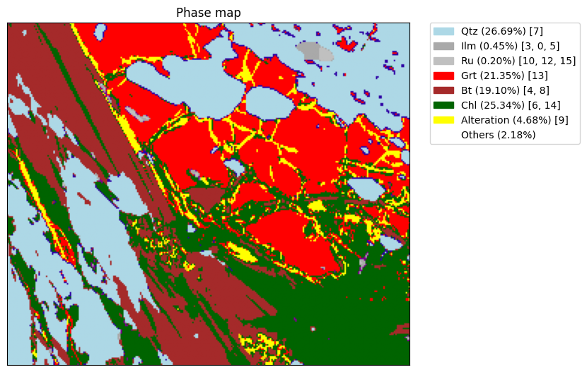
EDS maps

from epmatools.maps import MapStore

h5 = MapStore.from_examples('ex1')
h5.samples

['Demo']

s = h5.get_sample('Demo')

s.show()

s.show('Ca')

s.show('Fe/(Fe+Mg)')

s.phasemap()